Resources 🤝
- We're covering a lot of content very quickly. If you're overwhelmed, just know that
we're here to support you!
- Campuswire and office hours are your friends!
- Check the Resources tab of the course website for programming resources.
Agenda
- Means and medians.
- Lists.
- Arrays.
- Ranges.
Means and medians
Describing numerical data
- We now know how to store individual numbers (as
ints orfloats) and pieces of text (as strings). But we often we'll work with sequences, or ordered collections, of several data values.
- For any collection of numbers, say temperatures, it can be helpful to summarize the data by its mean (i.e. average) or median.
- Both mean and median are measures of central tendency – that is, they tell us roughly where the "center" of the data falls.
The mean (i.e. average)
The mean is a one-number summary of a collection of numbers.
For example, the mean of $1$, $4$, $7$, and $12$ is $\frac{1 + 4 + 7 + 12}{4} = 6$.
Observe that the mean:
- Doesn't have to be equal to one of the data points.
- Doesn't have to be an integer, even if all of the data points are integers.
- Is somewhere between the min and max, but not necessarily halfway between.
- Has the same units as the data.
The median
Like the mean, the median is a one-number summary of a collection of numbers.
- To calculate it, sort the data points and pick the number in the middle.
- If there are two middle numbers, we usually pick the number halfway between (i.e. the mean of the middle two).
- Example:
- $\text{Median}(1, 4, 7, 12, 32) = 7$
- $\text{Median}(1, 4, 7, 12) = 5.5$
Mean vs. median
- The mean and median of a dataset can be the same, but they don't need to be. They measure the center of a dataset in two different ways.
- Two different datasets can have the same mean without having the same median, and vice versa.
Activity
-
Find two different datasets that have the same mean and different medians.
-
Find two different datasets that have the same median and different means.
-
Find two different datasets that have the same median and the same mean.
Means and medians are just summaries; they don't tell the whole story about a dataset!
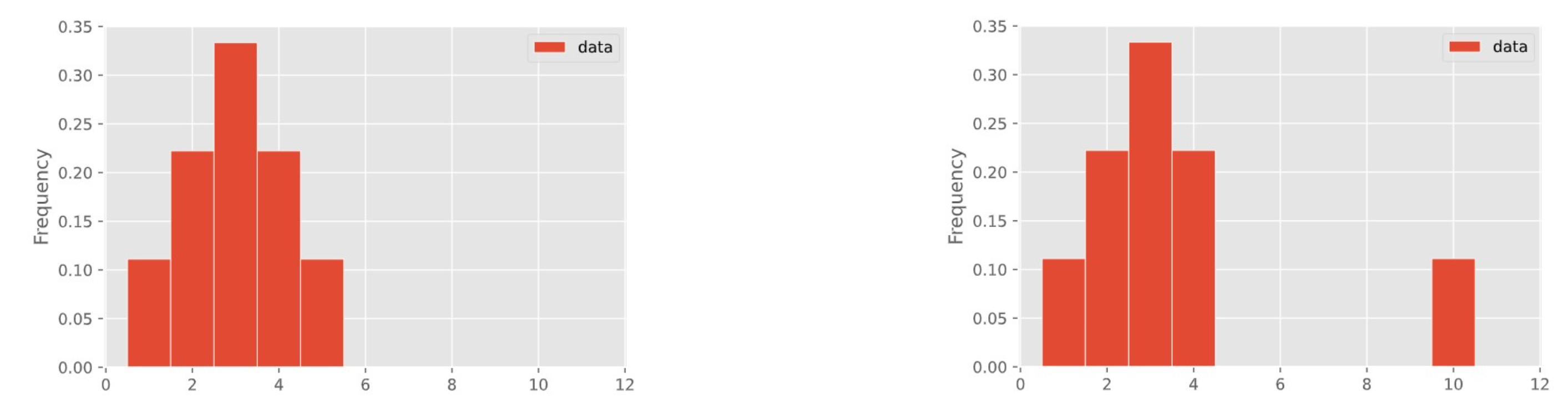
In a few weeks, we'll learn about how to visualize the distribution of a collection of numbers using a histogram.
These two distributions have different means but the same median!
Lists
Average temperature for a week
How would we store the temperatures for a week to compute the average temperature?
Our best solution right now is to create a separate variable for each day of the week.
temp_sunday = 68
temp_monday = 73
temp_tuesday = 70
temp_wednesday = 74
temp_thursday = 76
temp_friday = 72
temp_saturday = 74
This technically allows us to do things like compute the average temperature:
avg_temperature = 1/7 * (
    temp_sunday
    + temp_monday
    + temp_tuesday
    + ...)
Imagine a whole month's data, or a whole year's data. It seems like we need a better solution.
Lists in Python
In Python, a list is used to store multiple values within a single variable. To create a new list from
scratch, we use [square brackets].
temperature_list = [68, 73, 70, 74, 76, 72, 74]
len(temperature_list)
7
Notice that the elements in a list don't need to be unique!
Lists make working with sequences easy!
To find the average temperature, we just need to divide the sum of the temperatures by the number of temperatures recorded:
temperature_list
[68, 73, 70, 74, 76, 72, 74]
sum(temperature_list) / len(temperature_list)
72.42857142857143
Types
The type of a list is... list.
temperature_list
[68, 73, 70, 74, 76, 72, 74]
type(temperature_list)
list
Within a list, you can store elements of different types.
mixed_list = [-2, 2.5, 'ucsd', [1, 3]]
mixed_list
[-2, 2.5, 'ucsd', [1, 3]]
There's a problem...
- Lists are very slow.
- This is not a big deal when there aren't many entries, but it's a big problem when there are millions or billions of entries.
Arrays
NumPy

-
NumPy (pronounced "num pie") is a Python library (module) that provides support for arrays and operations on them.
-
The
babypandaslibrary, which you will learn about soon, goes hand-in-hand with NumPy.- NumPy is used heavily in the real world.
-
To use
numpy, we need to import it. It's usually imported asnp(but doesn't have to be!)
import numpy as np
Arrays
Think of NumPy arrays (just "arrays" from now on) as fancy, faster lists.

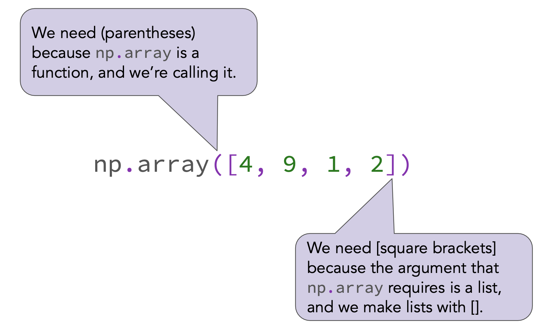
To create an array, we pass a list as input to the np.array function.
np.array([4, 9, 1, 2])
array([4, 9, 1, 2])
temperature_array = np.array([68, 73, 70, 74, 76, 72, 74])
temperature_array
array([68, 73, 70, 74, 76, 72, 74])
temperature_list
[68, 73, 70, 74, 76, 72, 74]
# No square brackets, because temperature_list is already a list!
np.array(temperature_list)
array([68, 73, 70, 74, 76, 72, 74])
Positions
When people wait in line, each person has a position.

Similarly, each element of an array (and list) has a position.
Accessing elements by position
- Python, like most programming languages, is "0-indexed."
- This means that the position of the first element in an array is 0, not 1.
- One interpretation is that an element's position represents the number of elements in front of it.
- To access the element in array
arr_nameat positionpos, we use the syntaxarr_name[pos].
temperature_array
array([68, 73, 70, 74, 76, 72, 74])
# If a position is negative, count from the end!
temperature_array[-2]
np.int64(72)
Types
Earlier in the lecture, we saw that lists can store elements of multiple types.
nums_and_strings_lst = ['uc', 'sd', 1961, 3.14]
nums_and_strings_lst
['uc', 'sd', 1961, 3.14]
This is not true of arrays – all elements in an array must be of the same type.
# All elements are converted to strings!
np.array(nums_and_strings_lst)
array(['uc', 'sd', '1961', '3.14'], dtype='<U32')
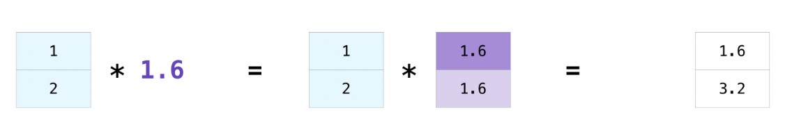
Array-number arithmetic
Arrays make it easy to perform the same operation to every element. This behavior is formally known as "broadcasting".
temperature_array
array([68, 73, 70, 74, 76, 72, 74])
# Increase all temperatures by 3 degrees.
temperature_array + 3
array([71, 76, 73, 77, 79, 75, 77])
# Halve all temperatures.
temperature_array / 2
array([34. , 36.5, 35. , 37. , 38. , 36. , 37. ])
# Convert all temperatures to Celsius.
(5 / 9) * (temperature_array - 32)
array([20.        , 22.77777778, 21.11111111, 23.33333333, 24.44444444,
       22.22222222, 23.33333333])
Note: In none of the above cells did we actually modify temperature_array!
Each of those expressions created a new array.
temperature_array
array([68, 73, 70, 74, 76, 72, 74])
To actually change temperature_array, we need to reassign it to a new array.
temperature_array = (5 / 9) * (temperature_array - 32)
# Now in Celsius!
temperature_array
array([20.        , 22.77777778, 21.11111111, 23.33333333, 24.44444444,
       22.22222222, 23.33333333])
Element-wise arithmetic
- We can apply arithmetic operations to multiple arrays, provided they have the same length.
- The result is computed element-wise, which means that the arithmetic operation is applied to one pair of elements from each array at a time.
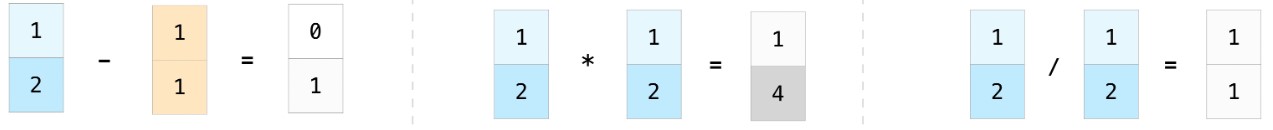
a = np.array([4, 5, -1])
b = np.array([2, 3, 2])
a + b
array([6, 8, 1])
a / b
array([ 2. , 1.66666667, -0.5 ])
a ** 2 + b ** 2
array([20, 34, 5])
Array methods
-
Arrays work with a variety of methods, which are functions designed to operate specifically on arrays.
-
Call these methods using dot notation, e.g.
array_name.method().
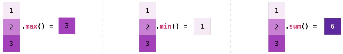
temperature_array.max()
np.float64(24.444444444444446)
temperature_array.mean()
np.float64(22.460317460317462)
Ranges
Motivation
We often find ourselves needing to make arrays like this:
day_of_month = np.array([
    1, 2, 3, 4, 5, 6, 7, 8, 9, 10, 11, 12,
    13, 14, 15, 16, 17, 18, 19, 20, 21, 22,
    23, 24, 25, 26, 27, 28, 29, 30, 31
])
There needs to be an easier way to do this!
Ranges
- A range is an array of evenly spaced numbers. We create ranges using
np.arange. - The most general way to create a range is
np.arange(start, end, step). This returns an array such that:- The first number is
start. By default,startis 0. - All subsequent numbers are spaced out by
step, until (but excluding)end. By default,stepis 1.
- The first number is
# Start at 0, end before 8, step by 1.
# This will be our most common use-case!
np.arange(8)
array([0, 1, 2, 3, 4, 5, 6, 7])
# Start at 5, end before 10, step by 1.
np.arange(5, 10)
array([5, 6, 7, 8, 9])
# Start at 3, end before 32, step by 5.
np.arange(3, 32, 5)
array([ 3, 8, 13, 18, 23, 28])
Extra practice
The step size in np.arange can be fractional, or even negative. Predict what arrays will be
produced by each line of code below. Then copy each line into a code cell and run it to see if you're
right.
np.arange(-3, 2, 0.5)

np.arange(1, -10, -3)
...
Ellipsis
...
Ellipsis
Challenge
🎉 Congrats! 🎉 You won the lottery 💰. Here's how your payout works: on the first day of September, you are paid \$0.01. Every day thereafter, your pay doubles, so on the second day you're paid \$0.02, on the third day you're paid \$0.04, on the fourth day you're paid \$0.08, and so on.
September has 30 days.
Write a one-line expression that uses the numbers 2 and 30,
along with the function np.arange and the method .sum(), that computes the total
amount in dollars you will be paid in September.
...
Ellipsis
After trying the challenge problem on your own, watch this walkthrough 🎥 video.
Summary, next time
Summary
- Lists and arrays are used to store sequences.
- Arrays are faster and more convenient for numerical operations.
- Arrays make it easy to perform arithmetic operations on all elements of an array and to perform element-wise operations on multiple arrays.
- Access elements by position, starting at position 0.
- Ranges are arrays of equally-spaced numbers. We create ranges with the function
np.arange.
Next time
We'll see how to use Python to work with real-world tabular data (data you might otherwise work with in a spreadsheet). This is where it gets fun!
Reminders
- Attend discussion section this afternoon at 2PM over ZOOM.
- Complete the items in the Getting Started section of the syllabus by Tuesday, June 30th at 11:59PM.
- Then, work on the Pretest and Lab 0, both due Tuesday, June 30th at 11:59PM. Access assignments by clicking links from the homepage of dsc10.com.