# Run this cell to set up packages for lecture.
from lec18_imports import *

Lecture 18 – Choosing Sample Sizes, Statistical Models

DSC 10, Winter 2025

Agenda

• Recap: The Central Limit Theorem (CLT).
• Choosing sample sizes.
• Models.

Recap: The Central Limit Theorem

show_clt_slides()

The Central Limit Theorem

• The Central Limit Theorem (CLT) says that the probability distribution of the sum or mean of a large random sample drawn with replacement will be roughly normal, regardless of the distribution of the population from which the sample is drawn.

• The distribution of the sample mean is centered at the population mean, and its standard deviation is

$$\text{SD of Distribution of Possible Sample Means} = \frac{\text{Population SD}}{\sqrt{\text{sample size}}}$$

• When we collect a single sample, we won't know the population mean or SD, so we'll use the sample mean and SD as approximations.

• Key idea: The CLT allows us to estimate the distribution of the sample mean, given just a single sample, without having to bootstrap!

Concept Check ✅ – Answer at cc.dsc10.com

Which one of these histograms corresponds to the distribution of the sample mean for samples of size 100 drawn from a population with mean 50 and SD 20?

Confidence intervals for the population mean

A 95% confidence interval for the population mean is given by

$$ \left[\text{sample mean} - 2\cdot \frac{\text{sample SD}}{\sqrt{\text{sample size}}}, \text{sample mean} + 2\cdot \frac{\text{sample SD}}{\sqrt{\text{sample size}}} \right] $$

This CI doesn't require bootstrapping, and it only requires three numbers – the sample mean, the sample SD, and the sample size!

Bootstrapping vs. the CLT

Bootstrapping still has its uses!

	Bootstrapping	CLT
Pro	Works for many sample statistics (mean, median, standard deviation).	Only requires 3 numbers – the sample mean, sample SD, and sample size.
Con	Very computationally expensive (requires drawing many, many samples from the original sample).	Only works for the sample mean (and sum).

Choosing sample sizes

Polling

• You want to estimate the proportion of UCSD students that use Duolingo, which is the most popular language learning app.

• To do so, you will ask a random sample of UCSD students whether or not they use Duolingo.

• You want to create a confidence interval that has:
  • A 95% confidence level.
  • A width of at most 0.06.
    • The interval (0.21, 0.25) would be fine, but the interval (0.21, 0.28) would not.

Question: How big of a sample do you need? 🤔

Aside: Proportions are means!

• The sample we collect will consist of only two unique values:
  • 1, if the student uses Duolingo.
  • 0, if they don't.

• We're interested in the proportion of values in our sample that are 1.

• This proportion is the same as the mean of our sample!

• For instance, suppose our sample is $0, 1, 1, 0, 1$. Then $\frac{3}{5}$ of the values are $1$. The sample mean is

$$\frac{0 + 1 + 1 + 0 + 1}{5} = \frac{3}{5}$$

Key takeaway: The CLT applies in this case as well! The distribution of the proportion of 1s in our sample is roughly normal.

Our strategy

We will:

1. Collect a random sample.
2. Compute the sample mean (i.e., the proportion of people who say "yes").
3. Compute the sample standard deviation.
4. Construct a 95% confidence interval for the population mean:

$$ \left[ \text{sample mean} - 2\cdot \frac{\text{sample SD}}{\sqrt{\text{sample size}}}, \ \text{sample mean} + 2\cdot \frac{\text{sample SD}}{\sqrt{\text{sample size}}} \right] $$

Note that the width of our CI is the right endpoint minus the left endpoint:

$$ \text{width} = 4 \cdot \frac{\text{sample SD}}{\sqrt{\text{sample size}}} $$

Our strategy

• We want a CI whose width is at most 0.06.

$$\text{width} = 4 \cdot \frac{\text{sample SD}}{\sqrt{\text{sample size}}}$$

• The width of our confidence interval depends on two things: the sample SD and the sample size.

• If we know the sample SD, we can find the appropriate sample size by re-arranging the following inequality:

$$4 \cdot \frac{\text{sample SD}}{\sqrt{\text{sample size}}} \leq 0.06$$

$$\sqrt{\text{sample size}} \geq 4 \cdot \frac{\text{sample SD}}{0.06} \\ \implies \boxed{\text{sample size} \geq \left( 4 \cdot \frac{\text{sample SD}}{0.06} \right)^2}$$

• Problem: Before polling, we don't know the sample SD, because we don't have a sample! We don't know the population SD either.

• Solution: Find an upper bound – i.e. the largest possible value – for the sample SD and use that.

Upper bound for the standard deviation of a sample

• Without any information about the values in a sample, we can't make any guarantees about the standard deviation of the sample.

• However, in this case, we know that the only values in our sample will be 0 ("no") and 1 ("yes").

• In Homework 5, we introduce a formula for the standard deviation of a collection of 0s and 1s:

$$\text{SD of Collection of 0s and 1s} = \sqrt{(\text{Prop. of 0s}) \times (\text{Prop. of 1s})}$$

# Plot the SD of a collection of 0s and 1s with p proportion of Os.
p = np.arange(0, 1.01, 0.01)
sd = np.sqrt(p * (1 - p))
plt.plot(p, sd)
plt.xlabel('p')
plt.ylabel(r'$\sqrt{p(1-p)}$');

• Fact: The largest possible value of the SD of a collection of 0s and 1s is 0.5.
  • This happens when half the values are 0 and half are 1.

Choosing a sample size

• In the sample we will collect, the maximum possible SD is 0.5.

• Earlier, we saw that to construct a confidence interval with the desired confidence level and width, our sample size needs to satisfy:

$$\text{sample size} \geq \left( 4 \cdot \frac{\text{sample SD}}{0.06} \right)^2$$

• Notice that as the sample SD increases, the required sample size increases.

• By using the maximum possible SD above, we ensure that we collect a large enough sample, no matter what the population and sample look like.

Choosing a sample size

$$\text{sample size} \geq \left( 4 \cdot \frac{\text{sample SD}}{0.06} \right)^2$$

By substituting 0.5 for the sample size, we get

$$\text{sample size} \geq \left( 4 \cdot \frac{\text{0.5}}{0.06} \right)^2$$

While any sample size that satisfies the above inequality will give us a confidence interval that satisfies the necessary properties, it's time-consuming to gather larger samples than necessary. So, we'll pick the smallest sample size that satisfies the above inequality.

(4 * 0.5 / 0.06) ** 2

1111.1111111111113

Conclusion: We must sample 1112 people to construct a 95% CI for the population mean that is at most 0.06 wide.

Activity

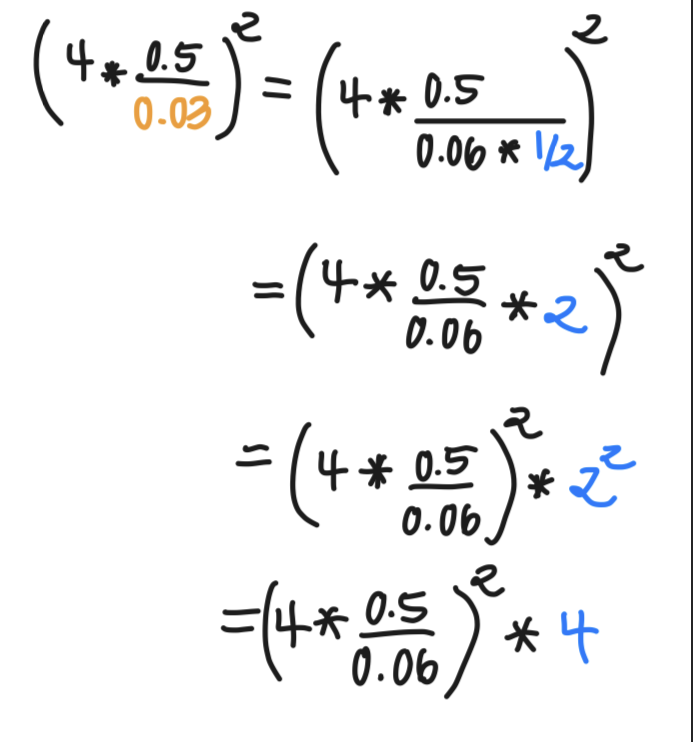
Suppose we instead want a 95% CI for the population mean that is at most 0.03 wide. What is the smallest sample size we could collect?

✅ Click here to see the answer after you've attempted the question yourself.

$$\text{sample size} \geq \left( 4 \cdot \frac{\text{0.5}}{0.03} \right)^2 = 4444.44$$

Therefore, the smallest sample size we could collect is 4445.

Statistical models

Statistical inference

• So far in the second half of this class, we've focused on the problem of parameter estimation.
  • Given a single sample, we can construct a confidence interval using bootstrapping (for most statistics) or the CLT (for the sample mean).
  • This confidence interval gives us a range of estimates for a parameter.

• Next, we'll turn our attention to answering yes-no questions about the relationships between samples and populations.
  • Example: Does it look like this jury panel was drawn randomly from this population of eligible jurors?
  • Example: Does it look like this sequence of coin tosses was generated by a fair coin?

• Both of these problems fall under the umbrella of statistical inference – using a sample to draw conclusions about the population.

Models

A model is a set of assumptions about how data was generated.

Example

Galileo's Leaning Tower of Pisa Experiment

Goal

• Our goal is to assess the quality of a model.

• Suppose we have access to a dataset. What we'll try to do is determine whether a model "explains" the patterns in the dataset.

Example: Jury selection

Swain vs. Alabama, 1965

• Robert Swain was a Black man convicted of crime in Talladega County, Alabama.

• He appealed the jury's decision all the way to the Supreme Court, on the grounds that Talladega County systematically excluded Black people from juries.

$\substack{\text{eligible} \\ \text{population}} \xrightarrow{\substack{\text{representative} \\ \text{sample}}} \substack{\text{jury} \\ \text{panel}} \xrightarrow{\substack{\text{selection by} \\ \text{judge/attorneys}}} \substack{\text{actual} \\ \text{jury}}$

• At the time, only men 21 years or older were allowed to serve on juries. 26% of this eligible population was Black.

• But of the 100 men on Robert Swain's jury panel, only 8 were Black.

Supreme Court ruling

• About disparities between the percentages in the eligible population and the jury panel, the Supreme Court wrote:

"... the overall percentage disparity has been small...”

• The Supreme Court denied Robert Swain’s appeal and he was sentenced to life in prison.

• We now have the tools to show quantitatively that the Supreme Court's claim was misguided.

• This "overall percentage disparity" turns out to be not so small, and is an example of racial bias.
  • Jury panels were often made up of people in the jury commissioner's professional and social circles.
  • Of the 8 Black men on the jury panel, none were selected to be part of the actual jury.

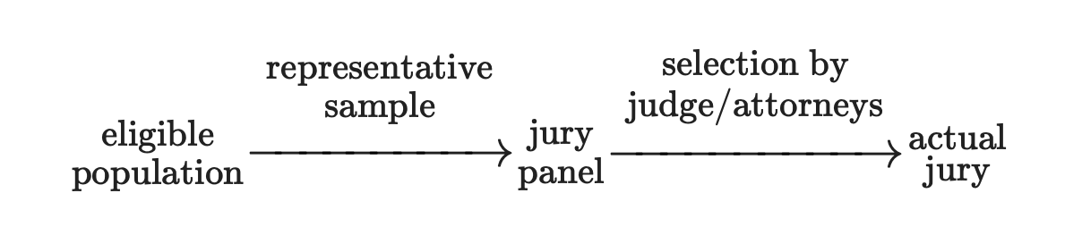
Setup

• Model: Jury panels consist of 100 men, randomly chosen from a population that is 26% Black.

• Observation: On the actual jury panel, only 8 out of 100 men were Black.

• Question: Does the model explain the observation?

Our approach: Simulation

• We'll start by assuming that the model is true.

• We'll generate many jury panels using this assumption.

• We'll count the number of Black men in each simulated jury panel to see how likely it is for a random panel to contain 8 or fewer Black men.
  • If we see 8 or fewer Black men often, then the model seems reasonable.
  • If we rarely see 8 or fewer Black men, then the model may not be reasonable.

Simulating statistics

Recall, a statistic is a number calculated from a sample.

Our plan:

1. Run an experiment once to generate one value of our chosen statistic.
   • In this case, sample 100 people randomly from a population that is 26% Black, and count the number of Black men (statistic).

2. Run the experiment many times, generating many values of the statistic, and store these statistics in an array.

3. Visualize the resulting empirical distribution of the statistic.

Step 1 – Running the experiment once

• How do we randomly sample a jury panel?
  • np.random.choice won't help us, because we don't know how large the eligible population is.

• The function np.random.multinomial helps us sample at random from a categorical distribution.

np.random.multinomial(sample_size, pop_distribution)

• np.random.multinomial samples at random from the population, with replacement, and returns a random array containing counts in each category.
  • pop_distribution needs to be an array containing the probabilities of each category.

Aside: Example usage of np.random.multinomial

On Halloween 👻, you trick-or-treated at 35 houses, each of which had an identical candy box, containing:

• 30% Starbursts.
• 30% Sour Patch Kids.
• 40% Twix.

At each house, you selected one candy blindly from the candy box.

To simulate the act of going to 35 houses, we can use np.random.multinomial:

np.random.multinomial(35, [0.3, 0.3, 0.4])

array([ 4, 11, 20])

Step 1 – Running the experiment once

In our case, a randomly selected member of our population is Black with probability 0.26 and not Black with probability 1 - 0.26 = 0.74.

demographics = [0.26, 0.74]

Each time we run the following cell, we'll get a new random sample of 100 people from this population.

• The first element of the resulting array is the number of Black men in the sample.
• The second element is the number of non-Black men in the sample.

np.random.multinomial(100, demographics)

array([25, 75])

Step 1 – Running the experiment once

We also need to calculate the statistic, which in this case is the number of Black men in the random sample of 100.

np.random.multinomial(100, demographics)[0]

25

Step 2 – Repeat the experiment many times

• Let's run 10,000 simulations.
• We'll keep track of the number of Black men in each simulated jury panel in the array counts.

counts = np.array([])

for i in np.arange(10000):
    new_count = np.random.multinomial(100, demographics)[0]
    counts = np.append(counts, new_count)
    
counts

array([30., 29., 28., ..., 27., 29., 28.])

Step 3 – Visualize the resulting distribution

Was a jury panel with 8 Black men suspiciously unusual?

(bpd.DataFrame().assign(count_black_men=counts)
                .plot(kind='hist', bins = np.arange(9.5, 45, 1), 
                      density=True, ec='w', figsize=(10, 5),
                      title='Empiricial Distribution of the Number of Black Men in Simulated Jury Panels of Size 100'));
observed_count = 8
plt.axvline(observed_count, color='black', linewidth=4, label='Observed Number of Black Men in Actual Jury Panel')
plt.legend();

# In 10,000 random experiments, the panel with the fewest Black men had how many?
counts.min()

11.0

Conclusion

• Our simulation shows that there's essentially no chance that a random sample of 100 men drawn from a population in which 26% of men are Black will contain 8 or fewer Black men.
• As a result, it seems that the model we proposed – that the jury panel was drawn at random from the eligible population – is flawed.
• There were likely factors other than chance that explain why there were only 8 Black men on the jury panel.

Summary, next time

Summary

• A 95% confidence interval for the population mean is given by

$$ \left[\text{sample mean} - 2\cdot \frac{\text{sample SD}}{\sqrt{\text{sample size}}}, \text{sample mean} + 2\cdot \frac{\text{sample SD}}{\sqrt{\text{sample size}}} \right] $$

• If we want to construct a confidence interval of a particular width and confidence level for a population proportion:
  1. Choose a confidence level (e.g. 95%) and maximum width (e.g. 0.06).
  2. Solve for the minimum sample size that satisfies both conditions.
  3. Collect a sample of that size.
  4. Use the formula above to construct an interval.
• A model is an assumption about how data was generated. We're interested in determining the validity a model, given some data we've collected.
• When assessing a model, we consider two viewpoints of the world: one where the model is true, and another where the model is false for some reason.

Next time

• Next time, we'll see more examples of testing models and deciding between two viewpoints.
• We'll formalize this notion, which is called hypothesis testing.