# Run this cell to set up packages for lecture.
from lec17_imports import *
Agenda
- Recap: Standard units.
- The Central Limit Theorem.
- Using the Central Limit Theorem to create confidence intervals.
Recap: Standard units
Standard units
Suppose $x$ is a numerical variable, and $x_i$ is one value of that variable. Then, $$x_{i \: \text{(su)}} = \frac{x_i - \text{mean of $x$}}{\text{SD of $x$}}$$
represents $x_i$ in standard units – the number of standard deviations $x_i$ is above the mean.
Activity: SAT scores
SAT scores range from 400 to 1600. The distribution of SAT scores has a mean of 1050 and a standard deviation of 200. Your friend tells you that their SAT score, in standard units, is 3.5. What do you conclude?
The Central Limit Theorem
Back to flight delays ✈️
The distribution of flight delays that we've been looking at is not roughly normal.
delays = bpd.read_csv('data/united_summer2015.csv')
delays.plot(kind='hist', y='Delay', bins=np.arange(-20.5, 210, 5), density=True, ec='w', figsize=(10, 5), title='Population Distribution of Flight Delays')
plt.xlabel('Delay (minutes)');

delays.get('Delay').describe()
count    13825.00
mean        16.66
std         39.48
           ...
50%          2.00
75%         18.00
max        580.00
Name: Delay, Length: 8, dtype: float64
Empirical distribution of a sample statistic
- Before we started discussing center, spread, and the normal distribution, our focus was on bootstrapping.
- We used bootstrapping to estimate the distribution of a sample statistic (e.g. sample mean or sample median), using just a single sample.
- We did this to construct confidence intervals for a population parameter.
- Important: For now, we'll suppose our parameter of interest is the population mean, so we're interested in estimating the distribution of the sample mean.
- What we're soon going to discover is a technique for finding the distribution of the sample mean and creating a confidence interval, without needing to bootstrap. Think of this as a shortcut to bootstrapping.
Empirical distribution of the sample mean
Since we have access to the population of flight delays, let's remind ourselves what the distribution of the sample mean looks like by drawing samples repeatedly from the population.
- This is not bootstrapping.
- This is also not practical. If we had access to a population, we wouldn't need to understand the distribution of the sample mean – we'd be able to compute the population mean directly.
sample_means = np.array([])
repetitions = 2000

for i in np.arange(repetitions):
    sample = delays.sample(500) # Not bootstrapping!
    sample_mean = sample.get('Delay').mean()
    sample_means = np.append(sample_means, sample_mean)

sample_means
array([19.19, 18.12, 13.52, ..., 15.17, 13.92, 16.3 ])
bpd.DataFrame().assign(sample_means=sample_means).plot(kind='hist', density=True, ec='w', alpha=0.65, bins=20, figsize=(10, 5));
plt.scatter([sample_means.mean()], [-0.005], marker='^', color='green', s=250)
plt.axvline(sample_means.mean(), color='green', label=f'mean={np.round(sample_means.mean(), 2)}', linewidth=4)
plt.xlim(5, 30)
plt.ylim(-0.013, 0.26)
plt.title('Distribution of the Sample Mean for Samples of Size 500')
plt.legend();

Notice that this distribution is roughly normal, even though the population distribution was not!
- This distribution is centered at the population mean.
- Can you estimate the standard deviation of this distribution using the inflection points?
The Central Limit Theorem
The Central Limit Theorem (CLT) says that the probability distribution of the sum or mean of a large random sample drawn with replacement* will be roughly normal, regardless of the distribution of the population from which the sample is drawn.
*If the population is infinite, then the CLT is true for sampling with or without replacement. Likewise, if the population is finite and the sample is sufficiently smaller than the population, it will not make much difference whether you sample with or without replacement.
While the formulas we're about to introduce only work for sample means, it's important to remember that the statement above also holds true for sample sums.
Characteristics of the distribution of the sample mean
- Shape: The CLT says that the distribution of the sample mean is roughly normal, no matter what the population looks like.
- Center: This distribution is centered at the population mean.
- Spread: What is the standard deviation of the distribution of the sample mean? How is it impacted by the sample size?
Changing the sample size
The function sample_mean_delays takes in an integer sample_size, and:
- Takes a sample of size
sample_sizedirectly from the population. - Computes the mean of the sample.
- Repeats steps 1 and 2 above 2000 times, and returns an array of the resulting means.
def sample_mean_delays(sample_size):
    sample_means = np.array([])
    for i in np.arange(2000):
        sample = delays.sample(sample_size)
        sample_mean = sample.get('Delay').mean()
        sample_means = np.append(sample_means, sample_mean)
    return sample_means
Let's call sample_mean_delays on several values of sample_size.
sample_means = {}
sample_sizes = [5, 10, 50, 100, 200, 400, 800, 1600]

for size in sample_sizes:
    sample_means[size] = sample_mean_delays(size)
Let's look at the resulting distributions.
plot_many_distributions(sample_sizes, sample_means)

What do you notice? 🤔
Standard deviation of the distribution of the sample mean
- As we increase our sample size, the distribution of the sample mean gets narrower, and so its standard deviation decreases.
- Can we determine exactly how much it decreases by?
# Compute the standard deviation of each distribution.
sds = np.array([])
for size in sample_sizes:
    sd = np.std(sample_means[size])
    sds = np.append(sds, sd)
sds
array([17.59, 11.6 , 5.49, 3.92, 2.8 , 1.95, 1.36, 0.91])
observed = bpd.DataFrame().assign(
    SampleSize=sample_sizes,
    StandardDeviation=sds
)

observed.plot(kind='scatter', x='SampleSize', y='StandardDeviation', s=70, title="Standard Deviation of the Distribution of the Sample Mean vs. Sample Size", figsize=(10, 5));

It appears that as the sample size increases, the standard deviation of the distribution of the sample mean decreases quickly.
Standard deviation of the distribution of the sample mean
- As we increase our sample size, the distribution of the sample mean gets narrower, and so its standard deviation decreases.
- Here's the mathematical relationship describing this phenomenon:
$$\text{SD of Distribution of Possible Sample Means} = \frac{\text{Population SD}}{\sqrt{\text{sample size}}}$$
- This is sometimes called the square root law. Its proof is outside the scope of this class; you'll see it if you take an upper-division probability course.
- This says that when we take large samples, the distribution of the sample mean is narrow, and so the sample mean is typically pretty close to the population mean. As expected, bigger samples tend to yield better estimates of the population mean.
- Note: This is not saying anything about the standard deviation of a sample itself! It is a statement about the distribution of all possible sample means. If we increase the size of the sample we're taking:
- It is not true ❌ that the SD of our sample will decrease.
- It is true ✅ that the SD of the distribution of all possible sample means of that size will decrease.
Recap: Distribution of the sample mean
Suppose we were to take many, many samples of the same size from a population, and take the mean of each sample. Then the distribution of the sample mean will have the following characteristics:
- Shape: The distribution will be roughly normal, regardless of the shape of the population distribution.
- Center: The distribution will be centered at the population mean.
- Spread: The distribution's standard deviation will be described by the square root law:
$$\text{SD of Distribution of Possible Sample Means} = \frac{\text{Population SD}}{\sqrt{\text{sample size}}}$$
🚨 Practical Issue: The mean and standard deviation of the distribution of the sample mean both depend on the original population, but we typically don't have access to the population!
Bootstrapping vs. the CLT
- The goal of bootstrapping was to estimate the distribution of a sample statistic (e.g. the sample mean), given just a single sample.
- The CLT describes the distribution of the sample mean, but it depends on information about the population (i.e. the population mean and population SD).
- Idea: The sample mean and SD are likely to be close to the population mean and SD. So, use them as approximations in the CLT!
- As a result, we can approximate the distribution of the sample mean, given just a single sample, without ever having to bootstrap!
- In other words, the CLT is a shortcut to bootstrapping!
Estimating the distribution of the sample mean by bootstrapping
Let's take a single sample of size 500 from delays.
np.random.seed(42)
my_sample = delays.sample(500)
my_sample.get('Delay').describe()
count    500.00
mean      13.01
std       28.00
          ...
50%        3.00
75%       16.00
max      209.00
Name: Delay, Length: 8, dtype: float64
Before today, to estimate the distribution of the sample mean using just this sample, we'd bootstrap:
resample_means = np.array([])
repetitions = 2000

for i in np.arange(repetitions):
    resample = my_sample.sample(500, replace=True) # Bootstrapping!
    resample_mean = resample.get('Delay').mean()
    resample_means = np.append(resample_means, resample_mean)

resample_means
array([12.65, 11.5 , 11.34, ..., 12.59, 11.89, 12.58])
bpd.DataFrame().assign(resample_means=resample_means).plot(kind='hist', density=True, ec='w', alpha=0.65, bins=20, figsize=(10, 5));
plt.scatter([resample_means.mean()], [-0.005], marker='^', color='green', s=250)
plt.axvline(resample_means.mean(), color='green', label=f'mean={np.round(resample_means.mean(), 2)}', linewidth=4)
plt.xlim(7, 20)
plt.ylim(-0.015, 0.35)
plt.legend();

The CLT tells us what this distribution will look like, without having to bootstrap!
Using the CLT with just a single sample
Now assume that all we have access to in practice is a single "original sample."
Suppose we were to bootstrap this original sample, which means we were to take many, many samples of the same size from this original sample, and take the mean of each resample. Then the distribution of the (re)sample mean will have the following characteristics:
- Shape: The distribution will be roughly normal, regardless of the shape of the original sample's distribution.
- Center: The distribution will be centered at the original sample's mean, which should be close to the population's mean.
- Spread: The distribution's standard deviation will be described by the square root law:
$$\begin{align} \text{SD of Distribution of Possible Sample Means} &= \frac{\text{Population SD}}{\sqrt{\text{sample size}}} \\ &\approx \boxed{\frac{\textbf{Sample SD}}{\sqrt{\text{sample size}}}} \end{align}$$
Let's test this out!
Using the CLT with just a single sample
Using just the original sample, my_sample, we estimate that the distribution of the sample mean has the following mean:
sample_mean_mean = my_sample.get('Delay').mean()
sample_mean_mean
13.008
and the following standard deviation:
sample_mean_sd = np.std(my_sample.get('Delay')) / np.sqrt(my_sample.shape[0])
sample_mean_sd
1.2511114546674091
Let's draw a normal distribution with the above mean and standard deviation, and overlay the bootstrapped distribution from earlier.
norm_x = np.linspace(7, 20)
norm_y = normal_curve(norm_x, mu=sample_mean_mean, sigma=sample_mean_sd)
bpd.DataFrame().assign(Bootstrapping=resample_means).plot(kind='hist', density=True, ec='w', alpha=0.65, bins=20, figsize=(10, 5));
plt.plot(norm_x, norm_y, color='black', linestyle='--', linewidth=4, label='CLT')
plt.title('Distribution of the Sample Mean, Using Two Methods')
plt.xlim(7, 20)
plt.legend();

Key takeaway: Given just a single sample, we can use the CLT to estimate the distribution of the sample mean, without bootstrapping.
show_clt_slides()
Why?
Now, we can make confidence intervals for population means without needing to bootstrap!
Confidence intervals
Confidence intervals
- Previously, we bootstrapped to construct confidence intervals.
- Strategy: Collect one sample, repeatedly resample from it, calculate the statistic on each resample, and look at the middle 95% of resampled statistics.
- But, if our statistic is the mean, we can use the CLT.
- Computationally cheaper – no simulation required!
- In both cases, we use just a single sample to construct our confidence interval.
Constructing a 95% confidence interval through bootstrapping
We already have a single sample, my_sample. Let's bootstrap to generate 2000 resample means.
my_sample.get('Delay').describe()
count    500.00
mean      13.01
std       28.00
          ...
50%        3.00
75%       16.00
max      209.00
Name: Delay, Length: 8, dtype: float64
resample_means = np.array([])
repetitions = 2000

for i in np.arange(repetitions):
    resample = my_sample.sample(500, replace=True)
    resample_mean = resample.get('Delay').mean()
    resample_means = np.append(resample_means, resample_mean)

resample_means
array([14.37, 13.93, 11.34, ..., 16.84, 14.46, 11.4 ])
bpd.DataFrame().assign(resample_means=resample_means).plot(kind='hist', density=True, ec='w', alpha=0.65, bins=20, figsize=(10, 5));
plt.scatter([resample_means.mean()], [-0.005], marker='^', color='green', s=250)
plt.axvline(resample_means.mean(), color='green', label=f'mean={np.round(resample_means.mean(), 2)}', linewidth=4)
plt.xlim(7, 20)
plt.ylim(-0.015, 0.35)
plt.legend();

One approach to computing a confidence interval for the population mean involves taking the middle 95% of this distribution.
left_boot = np.percentile(resample_means, 2.5)
right_boot = np.percentile(resample_means, 97.5)
[left_boot, right_boot]
[10.6359, 15.61205]
bpd.DataFrame().assign(resample_means=resample_means).plot(kind='hist', y='resample_means', alpha=0.65, bins=20, density=True, ec='w', figsize=(10, 5), title='Distribution of Bootstrapped Sample Means');
plt.plot([left_boot, right_boot], [0, 0], color=gold, linewidth=12, label='95% bootstrap-based confidence interval');
plt.xlim(7, 20);
plt.legend();

Middle 95% of a normal distribution
But we didn't need to bootstrap to learn what the distribution of the sample mean looks like. We could instead use the CLT, which tells us that the distribution of the sample mean is normal. Further, its mean and standard deviation are approximately:
sample_mean_mean = my_sample.get('Delay').mean()
sample_mean_mean
13.008
sample_mean_sd = np.std(my_sample.get('Delay')) / np.sqrt(my_sample.shape[0])
sample_mean_sd
1.2511114546674091
So, the distribution of the sample mean is approximately:
draw_normal_curve(sample_mean_mean, sample_mean_sd)

Question: What interval on the $x$-axis captures the middle 95% of this distribution?
Recall: Proportion of values within $z$ SDs of the mean
| Range | All Distributions (via Chebyshev's inequality) | Normal Distribution |
|---|---|---|
| mean $\pm \ 1$ SD | $\geq 0\%$ | $\approx 68\%$ |
| mean $\pm \ 2$ SDs | $\geq 75\%$ | $\approx 95\%$ |
| mean $\pm \ 3$ SDs | $\geq 88.8\%$ | $\approx 99.73\%$ |
As we saw last class, if a variable is roughly normal, then approximately 95% of its values are within 2 standard deviations of its mean.
normal_area(-2, 2)

stats.norm.cdf(2) - stats.norm.cdf(-2)
0.9544997361036416
Let's use this fact here!
Computing a 95% confidence interval using the CLT
- Approximately 95% of a normal distribution's values fall within $\pm$ 2 SDs of the mean.
- The distribution in question here is the distribution of the sample mean. Don't confuse the sample SD with the SD of the sample mean's distribution!
$$\text{SD of Distribution of Possible Sample Means} \approx \frac{\text{Sample SD}}{\sqrt{\text{sample size}}}$$
- So, our interval is given by:
$$ \left[\text{sample mean} - 2\cdot \frac{\text{sample SD}}{\sqrt{\text{sample size}}}, \text{sample mean} + 2\cdot \frac{\text{sample SD}}{\sqrt{\text{sample size}}} \right] $$
left_normal = sample_mean_mean - 2 * sample_mean_sd
right_normal = sample_mean_mean + 2 * sample_mean_sd
[left_normal, right_normal]
[10.50577709066518, 15.510222909334818]
Visualizing the CLT-based confidence interval
plt.figure(figsize=(10, 5))
norm_x = np.linspace(7, 20)
norm_y = normal_curve(norm_x, mu=sample_mean_mean, sigma=sample_mean_sd)
plt.plot(norm_x, norm_y, color='black', linestyle='--', linewidth=4, label='Distribution of the Sample Mean (via the CLT)')
plt.xlim(7, 20)
plt.ylim(0, 0.41)
plt.plot([left_normal, right_normal], [0, 0], color='#8f6100', linewidth=12, label='95% CLT-based confidence interval')
plt.legend();

Comparing confidence intervals
We've constructed two confidence intervals for the population mean:
One using bootstrapping,
[left_boot, right_boot]
[10.6359, 15.61205]
and one using the CLT.
[left_normal, right_normal]
[10.50577709066518, 15.510222909334818]
In both cases, we only used information in my_sample, not the population.
The intervals created using each method are slightly different because both methods tried to approximate the true distribution of the sample mean in different ways.
- The CLT-based interval was created using the mean and SD of the sample, rather than the population. (Also, the true percentage of values that fall within 2 SDs of the mean in a normal distribution is slightly more than 95%.)
- The bootstrap-based interval depended on many random resamples from the original sample.
Recap: Confidence intervals for the population mean
A 95% confidence interval for the population mean is given by
$$ \left[\text{sample mean} - 2\cdot \frac{\text{sample SD}}{\sqrt{\text{sample size}}}, \text{sample mean} + 2\cdot \frac{\text{sample SD}}{\sqrt{\text{sample size}}} \right] $$
This CI doesn't require bootstrapping, and it only requires three numbers – the sample mean, the sample SD, and the sample size!
Bootstrapping vs. the CLT
Bootstrapping still has its uses!
| Bootstrapping | CLT | |
|---|---|---|
| Pro | Works for many sample statistics (mean, median, standard deviation). |
Only requires 3 numbers – the sample mean, sample SD, and sample size. |
| Con | Very computationally expensive (requires drawing many, many samples from the original sample). |
Only works for the sample mean (and sum). |
Note: At least for our purposes, there is no specific "minimum sample size" necessary to use either tool.
Activity
We just saw that when $z = 2$, the following is a 95% confidence interval for the population mean.
$$ \left[\text{sample mean} - z\cdot \frac{\text{sample SD}}{\sqrt{\text{sample size}}}, \text{sample mean} + z\cdot \frac{\text{sample SD}}{\sqrt{\text{sample size}}} \right] $$
Question: What value of $z$ should we use to create an 80% confidence interval? 90%?
estimate_z()
HBox(children=(FloatSlider(value=2.0, description='z', max=4.0, step=0.05),))
Output()
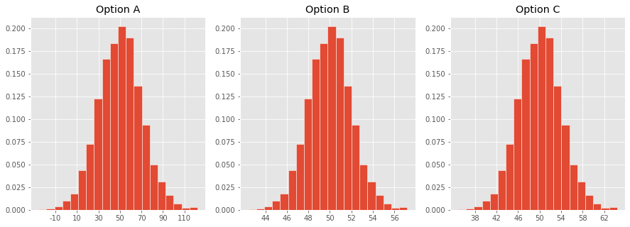
Concept Check ✅ – Answer at cc.dsc10.com
Which one of these histograms corresponds to the distribution of the sample mean for samples of size 100 drawn from a population with mean 50 and SD 20?
Summary, next time
Summary
- The Central Limit Theorem (CLT) says that the probability distribution of the sum or mean of a large random sample drawn with replacement will be roughly normal, regardless of the distribution of the population from which the sample is drawn.
- In the case of the sample mean, the CLT says:
- The distribution of the sample mean is centered at the population mean.
- The SD of the distribution of the sample mean is $\frac{\text{Population SD}}{\sqrt{\text{sample size}}}$.
- A 95% CLT-based confidence interval for the population mean is given by
$$ \left[\text{sample mean} - 2\cdot \frac{\text{sample SD}}{\sqrt{\text{sample size}}}, \text{sample mean} + 2\cdot \frac{\text{sample SD}}{\sqrt{\text{sample size}}} \right] $$
Next time
- Choosing sample sizes.
- We want to construct a confidence interval whose width is at most $w$. How many people should we sample?
- Moving away from parameter estimation, towards answering yes or no questions with hypothesis testing.