# Run this cell to set up packages for lecture.
from lec10_imports_1 import *

Lecture 10, Part 1: Finishing up bootstrapping and introduction to confidence Intervals

DSC 10, Summer 2025

Recap: Statistical inference

City of San Diego employee salary data

All City of San Diego employee salary data is public. We are using the latest available data.

population = bpd.read_csv('data/2023_salaries.csv')
population

	Year	EmployerType	EmployerName	DepartmentOrSubdivision	...	EmployerCounty	SpecialDistrictActivities	IncludesUnfundedLiability	SpecialDistrictType
0	2023	City	San Diego	Police	...	San Diego	NaN	False	NaN
1	2023	City	San Diego	Police	...	San Diego	NaN	False	NaN
2	2023	City	San Diego	Police	...	San Diego	NaN	False	NaN
...	...	...	...	...	...	...	...	...	...
13885	2023	City	San Diego	Transportation	...	San Diego	NaN	False	NaN
13886	2023	City	San Diego	Police	...	San Diego	NaN	False	NaN
13887	2023	City	San Diego	Public Utilities	...	San Diego	NaN	False	NaN

13888 rows × 29 columns

Note that unlike the previous histogram we saw, this is depicting the distribution of the population and of one particular sample (my_sample), not the distribution of sample medians for 1000 samples.

np.random.seed(38) # Magic to ensure that we get the same results every time this code is run.

# Take a sample of size 500.
my_sample = population.sample(500)
my_sample

	Year	EmployerType	EmployerName	DepartmentOrSubdivision	...	EmployerCounty	SpecialDistrictActivities	IncludesUnfundedLiability	SpecialDistrictType
4091	2023	City	San Diego	Engineering & Capital Projects	...	San Diego	NaN	False	NaN
2363	2023	City	San Diego	Public Utilities	...	San Diego	NaN	False	NaN
3047	2023	City	San Diego	Public Utilities	...	San Diego	NaN	False	NaN
...	...	...	...	...	...	...	...	...	...
4338	2023	City	San Diego	Parks & Recreation	...	San Diego	NaN	False	NaN
9238	2023	City	San Diego	Parks & Recreation	...	San Diego	NaN	False	NaN
4798	2023	City	San Diego	Development Services	...	San Diego	NaN	False	NaN

500 rows × 29 columns

Quick recap: Bootstrapping 🥾

Bootstrapping

• Shortcut: Use the sample in lieu of the population.
  • The sample itself looks like the population.
  • So, resampling from the sample is kind of like sampling from the population.
  • The act of resampling from a sample is called bootstrapping.

Bootstrapping the sample of salaries

We can simulate the act of collecting new samples by sampling with replacement from our original sample, my_sample.

# Note that the population DataFrame, population, doesn't appear anywhere here.
# This is all based on one sample, my_sample.

np.random.seed(38) # Magic to ensure that we get the same results every time this code is run.

n_resamples = 5000
boot_medians = np.array([])

for i in range(n_resamples):
    
    # Resample from my_sample WITH REPLACEMENT.
    resample = my_sample.sample(500, replace=True)
    
    # Compute the median.
    median = resample.get('TotalWages').median()
    
    # Store it in our array of medians.
    boot_medians = np.append(boot_medians, median)

boot_medians

array([85751. , 76009. , 83106. , ..., 82760. , 83470.5, 82711. ])

Bootstrap distribution of the sample median

# from last lecture
population_median = population.get('TotalWages').median()
population_median

80492.0

bpd.DataFrame().assign(BootstrapMedians=boot_medians).plot(kind='hist', density=True, bins=np.arange(65000, 95000, 1000), ec='w', figsize=(10, 5))
plt.scatter(population_median, 0.000004, color='blue', s=100, label='population median').set_zorder(2)
plt.legend();

The population median (blue dot) is near the middle.

In reality, we'd never get to see this!

What's the point of bootstrapping?

We have a sample median wage:

my_sample.get('TotalWages').median()

82508.0

With it, we can say that the population median wage is approximately \$82,508, and not much else.

But by bootstrapping our one sample, we can generate an empirical distribution of the sample median:

(bpd.DataFrame()
 .assign(BootstrapMedians=boot_medians)
 .plot(kind='hist', density=True, bins=np.arange(65000, 95000, 1000), ec='w', figsize=(10, 5))
)
plt.legend();

which allows us to say things like

We think the population median wage is between \$70,000 and \$88,000.

Question: We could also say that we think the population median wage is between \$80,000 and \$85,000. What range should we pick?

Percentiles

Informal definition

Let $p$ be a number between 0 and 100. The $p$th percentile of a numerical dataset is a number that's greater than or equal to $p$ percent of all data values.

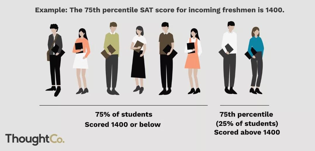
Another example: If you're in the $80$th percentile for height, it means that roughly $80\%$ of people are shorter than you, and $20\%$ are taller.

Calculating percentiles

• The numpy package provides a function to calculate percentiles, np.percentile(array, p), which returns the pth percentile of array.
• We won't worry about how this value is calculated - we'll just use the result!

np.percentile([4, 6, 9, 2, 7], 50) # unsorted data 

6.0

np.percentile([2, 4, 6, 7, 9], 50) # sorted data

6.0

Confidence intervals

Using the bootstrapped distribution of sample medians

Earlier in the lecture, we generated a bootstrapped distribution of sample medians.

bpd.DataFrame().assign(BootstrapMedians=boot_medians).plot(kind='hist', density=True, bins=np.arange(65000, 95000, 1000), ec='w', figsize=(10, 5))
plt.scatter(population_median, 0.000004, color='blue', s=100, label='population median').set_zorder(2)
plt.legend();

What can we do with this distribution, now that we know about percentiles?

Using the bootstrapped distribution of sample medians

• We have a sample median, \$82,508.

• As such, we think the population median is close to \$82,508. However, we're not quite sure how close.

• How do we capture our uncertainty about this guess?

• 💡 Idea: Find a range that captures most (e.g. 95%) of the bootstrapped distribution of sample medians. Such an interval is called a confidence interval.

Endpoints of a 95% confidence interval

• We want to find two points, $x$ and $y$, such that:
  • The area to the left of $x$ in the bootstrapped distribution is about 2.5%.
  • The area to the right of $y$ in the bootstrapped distribution is about 2.5%.

• The interval $[x,y]$ will contain about 95% of the total area, i.e. 95% of the total values. As such, we will call $[x, y]$ a 95% confidence interval.

• $x$ and $y$ are the 2.5th percentile and 97.5th percentile, respectively.

Finding the endpoints with np.percentile

boot_medians

array([85751. , 76009. , 83106. , ..., 82760. , 83470.5, 82711. ])

# Left endpoint.
left = np.percentile(boot_medians, 2.5)
left

70671.5

# Right endpoint.
right = np.percentile(boot_medians, 97.5)
right

86405.0

# Therefore, our interval is:
[left, right]

[70671.5, 86405.0]

You will use the code above very frequently moving forward!

Visualizing our 95% confidence interval

• Let's draw the interval we just computed on the histogram.
• 95% of the bootstrap medians fell into this interval.

bpd.DataFrame().assign(BootstrapMedians=boot_medians).plot(kind='hist', density=True, bins=np.arange(65000, 95000, 1000), ec='w', figsize=(10, 5), zorder=1)
plt.plot([left, right], [0, 0], color='gold', linewidth=12, label='95% confidence interval', zorder=2);
plt.scatter(population_median, 0.000004, color='blue', s=100, label='population median', zorder=3)
plt.legend();

• In this case, our 95% confidence interval (gold line) contains the true population parameter (blue dot).
  • It won't always, because you might have a bad original sample!
  • In reality, you won't know where the population parameter is, and so you won't know if your confidence interval contains it.

Concept Check ✅ – Answer at cc.dsc10.com

We computed the following 95% confidence interval:

print('Interval:', [left, right])
print('Width:', right - left)

Interval: [70671.5, 86405.0]
Width: 15733.5

If we instead computed an 80% confidence interval, would it be wider or narrower?

A. Wider                  B. Narrower                  C. Impossible to tell

Reflection

Now, instead of saying

We think the population median is close to our sample median, \$82,508.

We can say:

A 95% confidence interval for the population median is \$70,671.50 to \$86,405.

Some lingering questions: What does 95% confidence mean? What are we confident about? Is this technique always "good"?

Summary, next time

Summary

• Given a single sample, we want to estimate some population parameter using just one sample. One sample gives one estimate of the parameter. To get a sense of how much our estimate might have been different with a different sample, we need more samples.
  • In real life, sampling is expensive. You only get one sample!
• Key idea: The distribution of a sample looks a lot like the distribution of the population it was drawn from. So we can treat it like the population and resample from it.
• Each resample yields another estimate of the parameter. Taken together, many estimates give a sense of how much variability exists in our estimates, or how certain we are of any single estimate being accurate.
• Bootstrapping gives us a way to generate the empirical distribution of a sample statistic. From this distribution, we can create a $c$% confidence interval by taking the middle $c$% of values of the bootstrapped distribution.
• Such an interval allows us to quantify the uncertainty in our estimate of a population parameter.
  • Instead of providing just a single estimate of a population parameter, e.g. \$82,508, we can provide a range of estimates, e.g. \$70,671.50 to \$86,405.
  • Confidence intervals are used in a variety of fields to capture uncertainty. For instance, political researchers create confidence intervals for the proportion of votes their favorite candidate will receive, given a poll of voters.