# Set up packages for lecture. Don't worry about understanding this code, but
# make sure to run it if you're following along.
import numpy as np
import babypandas as bpd
import pandas as pd
from matplotlib_inline.backend_inline import set_matplotlib_formats
import matplotlib.pyplot as plt
from scipy import stats
set_matplotlib_formats("svg")
plt.style.use('ggplot')

np.set_printoptions(threshold=20, precision=2, suppress=True)
pd.set_option("display.max_rows", 7)
pd.set_option("display.max_columns", 8)
pd.set_option("display.precision", 2)

from ipywidgets import widgets
from IPython.display import clear_output, display

import warnings
warnings.filterwarnings('ignore')

# New minimize function (wrapper around scipy.optimize.minimize)
from inspect import signature
from scipy import optimize

def minimize(function):
    n_args = len(signature(function).parameters)
    initial = np.zeros(n_args)
    return optimize.minimize(lambda x: function(*x), initial).x

# All of the following code is for visualization.
def plot_regression_line(df, x, y, margin=.02):
    '''Computes the slope and intercept of the regression line between columns x and y in df (in original units) and plots it.'''
    m = slope(df, x, y)
    b = intercept(df, x, y)
    
    df.plot(kind='scatter', x=x, y=y, s=100, figsize=(10, 5), label='original data')
    left = df.get(x).min()*(1 - margin)
    right = df.get(x).max()*(1 + margin)
    domain = np.linspace(left, right, 10)
    plt.plot(domain, m*domain + b, color='orange', label='regression line', lw=4)
    plt.suptitle(format_equation(m, b), fontsize=18)
    plt.legend();
    
def format_equation(m, b):
    if b > 0:
        return r'$y = %.2fx + %.2f$' % (m, b)
    elif b == 0:
        return r'$y = %.2fx' % m
    else:
        return r'$y = %.2fx %.2f$' % (m, b)
    
def plot_errors(df, m, b, ax=None):
    x = df.get('x')
    y = m * x + b
    df.plot(kind='scatter', x='x', y='y', s=100, label='original data', ax=ax, figsize=(10, 5) if ax is None else None)
    
    if ax:
        plotter = ax
    else:
        plotter = plt
    
    plotter.plot(x, y, color='orange', lw=4)
    
    for k in np.arange(df.shape[0]):
        xk = df.get('x').iloc[k]
        yk = np.asarray(y)[k]
        if k == df.shape[0] - 1:
            plotter.plot([xk, xk], [yk, df.get('y').iloc[k]], linestyle=(0, (1, 1)), c='r', lw=4, label='errors')
        else:
            plotter.plot([xk, xk], [yk, df.get('y').iloc[k]], linestyle=(0, (1, 1)), c='r', lw=4)
    
    plt.title(format_equation(m, b), fontsize=18)
    plt.xlim(50, 90)
    plt.ylim(40, 100)
    plt.legend();

Lecture 24 – Regression and Least Squares

DSC 10, Winter 2023

Announcements

• Lab 7 is due tomorrow at 11:59 PM.
  • We'll drop the lowest lab, so you may not need to submit this if you've done well on all the others. However, this is the only assignment on regression, which will be tested on the final exam, so it's a good idea to do it for practice at least.
• The Final Project is due on Tuesday 3/14 at 11:59 PM.

Check-in ✅ – Answer at cc.dsc10.com

The Final Project is due on Tuesday 3/14 at 11:59 PM and has 8 sections. How much progress have you made?

A. Not started or barely started ⏳
B. Finished 1 or 2 sections
C. Finished 3 or 4 sections ❤️
D. Finished 5 or 6 sections
E. Finished 7 or 8 sections 🤯

Agenda

• The regression line, in standard units.
• The regression line, in original units.
• Outliers.
• Errors in prediction.

The regression line, in standard units

Example: Predicting heights 👪 📏

Recall, in the last lecture, we aimed to use a mother's height to predict her adult son's height.

galton = bpd.read_csv('data/galton.csv')
male_children = galton[galton.get('gender') == 'male']
mom_son = bpd.DataFrame().assign(mom = male_children.get('mother'), 
                                 son = male_children.get('childHeight'))
mom_son

	mom	son
0	67.0	73.2
4	66.5	73.5
5	66.5	72.5
...	...	...
925	60.0	66.0
929	66.0	64.0
932	63.0	66.5

481 rows × 2 columns

mom_son.plot(kind='scatter', x='mom', y='son', figsize=(10, 5));

Correlation

Recall, the correlation coefficient $r$ of two variables $x$ and $y$ is defined as the

• average value of the
• product of $x$ and $y$
• when both are measured in standard units.

def standard_units(any_numbers):
    "Convert a sequence of numbers to standard units."
    return (any_numbers - any_numbers.mean()) / np.std(any_numbers)

def correlation(df, x, y):
    "Computes the correlation between column x and column y of df."
    return (standard_units(df.get(x)) * standard_units(df.get(y))).mean()

r_mom_son = correlation(mom_son, 'mom', 'son')
r_mom_son

0.32300498368490554

The regression line

• The regression line is the line through $(0,0)$ with slope $r$, when both variables are measured in standard units.

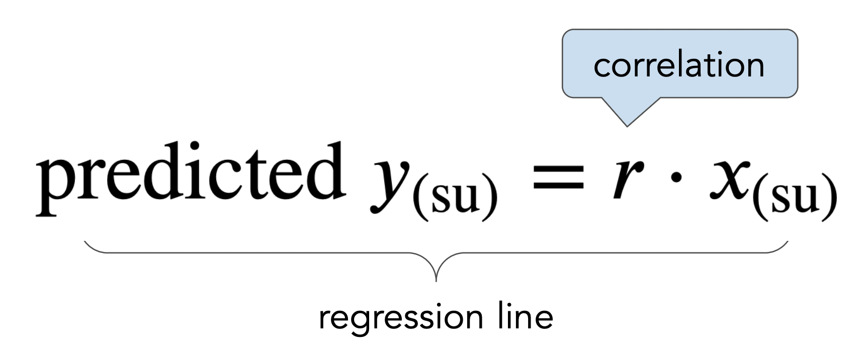
• We use the regression line to make predictions!

Making predictions in standard units

• If $r = 0.32$, and the given $x$ is $2$ in standard units, then the prediction for $y$ is $0.64$ standard units.
  • The regression line predicts that a mother whose height is $2$ SDs above average has a son whose height is $0.64$ SDs above average.

• We always predict that a son will be somewhat closer to average in height than his mother.
  • This is a consequence of the slope $r$ having magnitude less than 1.
  • This effect is called regression to the mean.

• The regression line passes through the origin $(0, 0)$ in standard units. This means that, no matter what $r$ is, for an average $x$ value, we predict an average $y$ value.

Making predictions in original units

Of course, we'd like to be able to predict a son's height in inches, not just in standard units. Given a mother's height in inches, here's how we'll predict her son's height in inches:

1. Convert the mother's height from inches to standard units.

$$x_{i \: \text{(su)}} = \frac{x_i - \text{mean of $x$}}{\text{SD of $x$}}$$

1. Multiply by the correlation coefficient to predict the son's height in standard units.

$$\text{predicted } y_{i \: \text{(su)}} = r \cdot x_{i \: \text{(su)}}$$

1. Convert the son's predicted height from standard units back to inches.

$$\text{predicted } y_i = \text{predicted } y_{i \: \text{(su)}} \cdot \text{SD of $y$} + \text{mean of $y$}$$

mom_mean = mom_son.get('mom').mean()
mom_sd = np.std(mom_son.get('mom'))
son_mean = mom_son.get('son').mean()
son_sd = np.std(mom_son.get('son'))

def predict_with_r(mom):
    """Return a prediction for the height of a son whose mother has height mom, 
    using linear regression.
    """
    mom_su = (mom - mom_mean) / mom_sd
    son_su = r_mom_son * mom_su
    return son_su * son_sd + son_mean

predict_with_r(68)

70.68219686848828

predict_with_r(60)

67.76170758654767

preds = mom_son.assign(
    predicted_height=mom_son.get('mom').apply(predict_with_r)
)
ax = preds.plot(kind='scatter', x='mom', y='son', title='Regression line predictions, in original units', figsize=(10, 5), label='original data')
preds.plot(kind='line', x='mom', y='predicted_height', ax=ax, color='orange', label='regression line', lw=4);
plt.legend();

Concept Check ✅ – Answer at cc.dsc10.com

A course has a midterm (mean 80, standard deviation 15) and a really hard final (mean 50, standard deviation 12).

If the scatter plot comparing midterm & final scores for students looks linearly associated with correlation 0.75, then what is the predicted final exam score for a student who received a 90 on the midterm?

• A. 54
• B. 56
• C. 58
• D. 60
• E. 62

The regression line, in original units

Reflection

Each time we wanted to predict the height of an adult son given the height of a mother, we had to:

1. Convert the mother's height from inches to standard units.

1. Multiply by the correlation coefficient to predict the son's height in standard units.

1. Convert the son's predicted height from standard units back to inches.

This is inconvenient – wouldn't it be great if we could express the regression line itself in inches?

From standard units to original units

When $x$ and $y$ are in standard units, the regression line is given by

What is the regression line when $x$ and $y$ are in their original units?

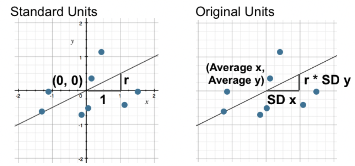
The regression line in original units

• We can work backwards from the relationship $$\text{predicted } y_{\text{(su)}} = r \cdot x_{\text{(su)}}$$ to find the line in original units.

$$\frac{\text{predicted } y - \text{mean of }y}{\text{SD of }y} = r \cdot \frac{x - \text{mean of } x}{\text{SD of }x}$$

• Note that $r, \text{mean of } x$, $\text{mean of } y$, $\text{SD of } x$, and $\text{SD of } y$ are constants – if you have a DataFrame with two columns, you can determine all 5 values.
• Re-arranging the above equation into the form $\text{predicted } y = mx + b$ yields the formulas:

$$m = r \cdot \frac{\text{SD of } y}{\text{SD of }x}, \: \: b = \text{mean of } y - m \cdot \text{mean of } x$$

• $m$ is the slope of the regression line and $b$ is the intercept.

Let's implement these formulas in code and try them out.

def slope(df, x, y):
    "Returns the slope of the regression line between columns x and y in df (in original units)."
    r = correlation(df, x, y)
    return r * np.std(df.get(y)) / np.std(df.get(x))

def intercept(df, x, y):
    "Returns the intercept of the regression line between columns x and y in df (in original units)."
    return df.get(y).mean() - slope(df, x, y) * df.get(x).mean()

Below, we compute the slope and intercept of the regression line between mothers' heights and sons' heights (in inches).

m_heights = slope(mom_son, 'mom', 'son')
m_heights

0.36506116024257595

b_heights = intercept(mom_son, 'mom', 'son')
b_heights

45.85803797199311

So, the regression line is

$$\text{predicted son's height} = 0.365 \cdot \text{mother's height} + 45.858$$

Making predictions

def predict_son(mom):
    return m_heights * mom + b_heights

What's the predicted height of a son whose mother is 62 inches tall?

predict_son(62)

68.49182990703282

What if the mother is 55 inches tall? 73 inches tall?

predict_son(55)

65.9364017853348

predict_son(73)

72.50750266970115

xs = np.arange(57, 72)
ys = predict_son(xs)
mom_son.plot(kind='scatter', x='mom', y='son', figsize=(10, 5), title='Regression line predictions, in original units', label='original data');
plt.plot(xs, ys, color='orange', lw=4, label='regression line')
plt.legend();

Outliers

The effect of outliers on correlation

Consider the dataset below. What is the correlation between $x$ and $y$?

outlier = bpd.read_csv('data/outlier.csv')
outlier.plot(kind='scatter', x='x', y='y', s=100, figsize=(10, 5));

correlation(outlier, 'x', 'y')

-0.02793982443854457

plot_regression_line(outlier, 'x', 'y')

Removing the outlier

without_outlier = outlier[outlier.get('y') > 40]

correlation(without_outlier, 'x', 'y')

0.9851437295364016

plot_regression_line(without_outlier, 'x', 'y')

Takeaway: Even a single outlier can have a massive impact on the correlation, and hence the regression line. Look for these before performing regression. Always visualize first!

Errors in prediction

Motivation

• We've presented the regression line in standard units as the line through the origin with slope $r$, given by $\text{predicted } y_{\text{(su)}} = r \cdot x_{\text{(su)}}$. Then, we used this equation to find a formula for the regression line in original units.

• In examples we've seen so far, the regression line seems to fit our data pretty well.
  • But how well?
  • What makes the regression line good?
  • Would another line be better?

Example: Without the outlier

outlier.plot(kind='scatter', x='x', y='y', s=100, figsize=(10, 5));

m_no_outlier = slope(without_outlier, 'x', 'y')
b_no_outlier = intercept(without_outlier, 'x', 'y')

m_no_outlier, b_no_outlier

(0.975927715724588, 3.042337135297444)

plot_errors(without_outlier, m_no_outlier, b_no_outlier)

We think our regression line is pretty good because most data points are pretty close to the regression line. The red lines are quite short.

Measuring the error in prediction

$$\text{error} = \text{actual value} - \text{prediction}$$

• Typically, some errors are positive and some negative.
  • What does a positive error mean? What about a negative error?

• To measure the rough size of the errors, for a particular set of predictions:
  1. Square the errors so that they don't cancel each other out.
  2. Take the mean of the squared errors.
  3. Take the square root to fix the units.

• This is called root mean square error (RMSE).
  • Notice the similarities to computing the SD!

Root mean squared error (RMSE) of the regression line's predictions

predictions = without_outlier.assign(pred=m_no_outlier * without_outlier.get('x') + b_no_outlier)
predictions = predictions.assign(diffs=predictions.get('y') - predictions.get('pred'))
predictions = predictions.assign(sq_diffs=predictions.get('diffs') ** 2)
predictions

	x	y	pred	diffs	sq_diffs
0	50	53.53	51.84	1.69	2.86
1	55	54.21	56.72	-2.51	6.31
2	60	65.65	61.60	4.06	16.45
...	...	...	...	...	...
6	80	79.61	81.12	-1.51	2.27
7	85	88.17	86.00	2.18	4.74
8	90	91.05	90.88	0.18	0.03

9 rows × 5 columns

np.sqrt(predictions.get('sq_diffs').mean())

2.19630831647554

The RMSE of the regression line's predictions is about 2.2. Is this big or small, relative to the predictions of other lines? 🤔