# Run this cell to set up packages for lecture.
from lec14_imports import *
Agenda
- Recap: Statistical inference.
- Bootstrapping 🥾.
- Percentiles.
- Confidence intervals.
Recap: Statistical inference
population = bpd.read_csv('data/2023_salaries.csv')
population
| Year | EmployerType | EmployerName | DepartmentOrSubdivision | ... | EmployerCounty | SpecialDistrictActivities | IncludesUnfundedLiability | SpecialDistrictType | |
|---|---|---|---|---|---|---|---|---|---|
| 0 | 2023 | City | San Diego | Police | ... | San Diego | NaN | False | NaN |
| 1 | 2023 | City | San Diego | Police | ... | San Diego | NaN | False | NaN |
| 2 | 2023 | City | San Diego | Police | ... | San Diego | NaN | False | NaN |
| ... | ... | ... | ... | ... | ... | ... | ... | ... | ... |
| 13885 | 2023 | City | San Diego | Transportation | ... | San Diego | NaN | False | NaN |
| 13886 | 2023 | City | San Diego | Police | ... | San Diego | NaN | False | NaN |
| 13887 | 2023 | City | San Diego | Public Utilities | ... | San Diego | NaN | False | NaN |
13888 rows × 29 columns
When you load in a dataset that has so many columns that you can't see them all, it's a good idea to look at the column names.
population.columns
Index(['Year', 'EmployerType', 'EmployerName', 'DepartmentOrSubdivision',
       'Position', 'ElectedOfficial', 'Judicial', 'OtherPositions',
       'MinPositionSalary', 'MaxPositionSalary', 'ReportedBaseWage',
       'RegularPay', 'OvertimePay', 'LumpSumPay', 'OtherPay', 'TotalWages',
       'DefinedBenefitPlanContribution', 'EmployeesRetirementCostCovered',
       'DeferredCompensationPlan', 'HealthDentalVision',
       'TotalRetirementAndHealthContribution', 'PensionFormula', 'EmployerURL',
       'EmployerPopulation', 'LastUpdatedDate', 'EmployerCounty',
       'SpecialDistrictActivities', 'IncludesUnfundedLiability',
       'SpecialDistrictType'],
      dtype='object')
We only need the 'TotalWages' column, so let's get just that column.
population = population.get(['TotalWages'])
population
| TotalWages | |
|---|---|
| 0 | 433011 |
| 1 | 416044 |
| 2 | 405315 |
| ... | ... |
| 13885 | 10 |
| 13886 | 8 |
| 13887 | 2 |
13888 rows × 1 columns
population.plot(kind='hist', bins=np.arange(0, 500000, 10000), density=True, ec='w', figsize=(10, 5),
                title='Distribution of Total Wages of San Diego City Employees in 2023');

The median salary
- We can use
.median()to find the median salary of all city employees. - This is a population parameter.
- This is not a random quantity.
population_median = population.get('TotalWages').median()
population_median
80492.0
Let's be realistic...
- In practice, it is costly and time-consuming to survey all the employees.
- More generally, we can't expect to survey all members of the population we care about.
- We happen to have the population here, but generally we won't.
- Instead, we gather salaries for a random sample of, say, 500 people.
Terminology recap
- The full DataFrame of salaries is the population.
- We observe a sample of 500 salaries from the population.
- We want to determine the population median (a parameter), but we don't have the whole population, so instead we use the sample median (a statistic) as an estimate.
- Hopefully the sample median is close to the population median.
Taking a sample
Let's survey 500 employees at random. To do so, we can use the .sample method.
np.random.seed(38) # Magic to ensure that we get the same results every time this code is run.

# Take a sample of size 500 without replacement (for 500 distinct individuals).
my_sample = population.sample(500)
my_sample
| TotalWages | |
|---|---|
| 4091 | 113944 |
| 2363 | 144835 |
| 3047 | 132502 |
| ... | ... |
| 4338 | 110628 |
| 9238 | 53840 |
| 4798 | 104600 |
500 rows × 1 columns
We won't reassign my_sample at any point in this notebook, so it will always refer to this particular sample.
my_sample.plot(kind='hist', bins=np.arange(0, 500000, 10000), density=True, ec='w', figsize=(10, 5),
                color = green, title='Distribution of Total Wages in a Sample of 500 City Employees');

# Compute the sample median.
sample_median = my_sample.get('TotalWages').median()
sample_median
82508.0
How confident are we that this is a good estimate?
- Our estimate depended on a random sample. If our sample was different, our estimate may have been different, too.
- How different could our estimate have been? Our confidence in the estimate depends on the answer to this question.
- The sample median is a random number. It comes from some distribution, which we don't know.
- If we did know what the distribution of the sample median looked like, it would help us determine how different our estimate might have been, if we'd drawn a different sample.
- "Narrow" distribution $\Rightarrow$ not too different.
- "Wide" distribution $\Rightarrow$ quite different.
An impractical approach
- One idea: repeatedly collect random samples of 500 from the population and compute their medians.
- This is what we did previously, to compute an empirical distribution of the sample mean of flight delays.
sample_medians = np.array([])
for i in np.arange(1000):
    median = population.sample(500).get('TotalWages').median()
    sample_medians = np.append(sample_medians, median)
sample_medians
array([82603.5, 84498. , 77594.5, ..., 83471.5, 84897.5, 75602. ])
(bpd.DataFrame()
 .assign(SampleMedians=sample_medians)
 .plot(kind='hist', density=True,
       bins=30, ec='w', figsize=(8, 5),
       title='Distribution of the Sample Median of 1000 Samples from the Population\nSample Size = 500')
);

- This shows an empirical distribution of the sample median. It is an approximation of the true probability distribution of the sample median, based on 1000 samples.
The problem
- Drawing new samples like this is impractical – we usually can't just ask for new samples from the population.
- If we were able to do this, why not just collect more data in the first place?
- Key insight: our original sample,
my_sample, looks a lot like the population.- Their distributions are similar.
fig, ax = plt.subplots(figsize=(10, 5))
bins=np.arange(10_000, 500_000, 10_000)
population.plot(kind='hist', y='TotalWages', ax=ax, density=True, alpha=.75, bins=bins, ec='w')
my_sample.plot(kind='hist', y='TotalWages', ax=ax, density=True, alpha=.75, bins=bins, ec='w')
plt.legend(['Population', 'My Sample']);

Note that unlike the previous histogram we saw, this is depicting the distribution of the population and of one particular sample (my_sample), not the distribution of sample medians for 1000 samples.
Bootstrapping 🥾
Bootstrapping
- Shortcut: Use the sample in lieu of the population.
- The sample itself looks like the population.
- So, resampling from the sample is kind of like sampling from the population.
- The act of resampling from a sample is called bootstrapping.
- In our case specifically:
- We have a sample of 500 salaries.
- We want another sample of 500 salaries, but we can't draw from the population.
- However, the original sample looks like the population.
- So, let's just resample from the sample!
show_bootstrapping_slides()
To replace or not replace?
- Our goal when bootstrapping is to create a sample of the same size as our original sample.
- Let's repeatedly resample 3 numbers without replacement from an original sample of [7, 9, 4].
original = [7, 9, 4]
for i in np.arange(10):
    resample = np.random.choice(original, 3, replace=False)
    print("Resample: ", resample, "    Median: ", np.median(resample))
Resample:  [9 4 7]     Median:  7.0
Resample:  [7 4 9]     Median:  7.0
Resample:  [4 7 9]     Median:  7.0
Resample:  [4 9 7]     Median:  7.0
Resample:  [7 4 9]     Median:  7.0
Resample:  [9 7 4]     Median:  7.0
Resample:  [4 7 9]     Median:  7.0
Resample:  [7 9 4]     Median:  7.0
Resample:  [9 4 7]     Median:  7.0
Resample:  [4 9 7]     Median:  7.0
- Let's repeatedly resample 3 numbers with replacement from an original sample of [7, 9, 4].
original = [7, 9, 4]
for i in np.arange(10):
    resample = np.random.choice(original, 3, replace=True)
    print("Resample: ", resample, "    Median: ", np.median(resample))
Resample:  [7 4 7]     Median:  7.0
Resample:  [9 4 9]     Median:  9.0
Resample:  [9 9 9]     Median:  9.0
Resample:  [9 4 9]     Median:  9.0
Resample:  [4 4 9]     Median:  4.0
Resample:  [9 9 7]     Median:  9.0
Resample:  [4 7 4]     Median:  4.0
Resample:  [9 4 7]     Median:  7.0
Resample:  [4 9 4]     Median:  4.0
Resample:  [7 4 4]     Median:  4.0
When we resample without replacement, resamples look just like the original samples.
When we resample with replacement, resamples can have a different mean, median, max, and min than the original sample.
- So, we need to sample with replacement to ensure that our resamples can be different from the original sample.
Bootstrapping the sample of salaries
We can simulate the act of collecting new samples by sampling with replacement from our original sample, my_sample.
# Note that the population DataFrame, population, doesn't appear anywhere here.
# This is all based on one sample, my_sample.

np.random.seed(38) # Magic to ensure that we get the same results every time this code is run.

n_resamples = 5000
boot_medians = np.array([])

for i in range(n_resamples):

    # Resample from my_sample WITH REPLACEMENT.
    resample = my_sample.sample(500, replace=True)

    # Compute the median.
    median = resample.get('TotalWages').median()

    # Store it in our array of medians.
    boot_medians = np.append(boot_medians, median)
boot_medians
array([85751. , 76009. , 83106. , ..., 82760. , 83470.5, 82711. ])
Bootstrap distribution of the sample median
bpd.DataFrame().assign(BootstrapMedians=boot_medians).plot(kind='hist', density=True, bins=np.arange(65000, 95000, 1000), ec='w', figsize=(10, 5))
plt.scatter(population_median, 0.000004, color=pink, s=100, label='population median').set_zorder(2)
plt.legend();

The population median (pink dot) is near the middle.
In reality, we'd never get to see this!
What's the point of bootstrapping?
We have a sample median wage:
my_sample.get('TotalWages').median()
82508.0
With it, we can say that the population median wage is approximately \$82,508, and not much else.
But by bootstrapping our one sample, we can generate an empirical distribution of the sample median:
(bpd.DataFrame()
 .assign(BootstrapMedians=boot_medians)
 .plot(kind='hist', density=True, bins=np.arange(65000, 95000, 1000), ec='w', figsize=(10, 5))
)
plt.legend();

which allows us to say things like
We think the population median wage is between \$70,000 and \$88,000.
Question: We could also say that we think the population median wage is between \$80,000 and \$85,000. What range should we pick?
Percentiles
Informal definition
Let $p$ be a number between 0 and 100. The $p$th percentile of a numerical dataset is a number that's greater than or equal to $p$ percent of all data values.
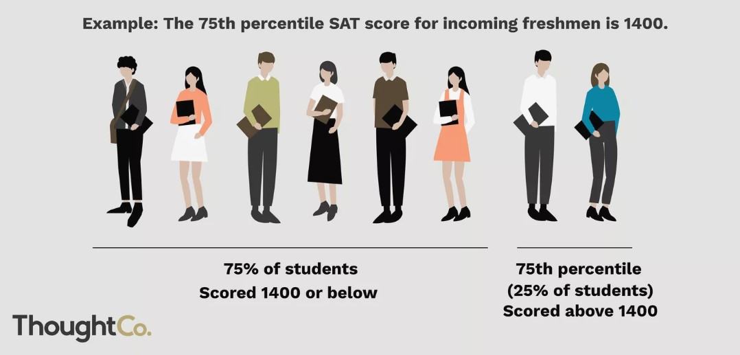
Another example: If you're in the $80$th percentile for height, it means that roughly $80\%$ of people are shorter than you, and $20\%$ are taller.

Calculating percentiles
- The
numpypackage provides a function to calculate percentiles,np.percentile(array, p), which returns thepth percentile ofarray. - We won't worry about how this value is calculated - we'll just use the result!
np.percentile([4, 6, 9, 2, 7], 50) # unsorted data
6.0
np.percentile([2, 4, 6, 7, 9], 50) # sorted data
6.0
Confidence intervals
Using the bootstrapped distribution of sample medians
Earlier in the lecture, we generated a bootstrapped distribution of sample medians.
bpd.DataFrame().assign(BootstrapMedians=boot_medians).plot(kind='hist', density=True, bins=np.arange(65000, 95000, 1000), ec='w', figsize=(10, 5))
plt.scatter(population_median, 0.000004, color=pink, s=100, label='population median').set_zorder(2)
plt.legend();
What can we do with this distribution, now that we know about percentiles?
Using the bootstrapped distribution of sample medians
- We have a sample median, \$82,508.
- As such, we think the population median is close to \$82,508. However, we're not quite sure how close.
- How do we capture our uncertainty about this guess?
- 💡 Idea: Find a range that captures most (e.g. 95%) of the bootstrapped distribution of sample medians. Such an interval is called a confidence interval.
Endpoints of a 95% confidence interval
- We want to find two points, $x$ and $y$, such that:
- The area to the left of $x$ in the bootstrapped distribution is about 2.5%.
- The area to the right of $y$ in the bootstrapped distribution is about 2.5%.
- The interval $[x,y]$ will contain about 95% of the total area, i.e. 95% of the total values. As such, we will call $[x, y]$ a 95% confidence interval.
- $x$ and $y$ are the 2.5th percentile and 97.5th percentile, respectively.
Finding the endpoints with np.percentile
boot_medians
array([85751. , 76009. , 83106. , ..., 82760. , 83470.5, 82711. ])
# Left endpoint.
left = np.percentile(boot_medians, 2.5)
left
70671.5
# Right endpoint.
right = np.percentile(boot_medians, 97.5)
right
86405.0
# Therefore, our interval is:
[left, right]
[70671.5, 86405.0]
You will use the code above very frequently moving forward!
Visualizing our 95% confidence interval
- Let's draw the interval we just computed on the histogram.
- 95% of the bootstrap medians fell into this interval.
bpd.DataFrame().assign(BootstrapMedians=boot_medians).plot(kind='hist', density=True, bins=np.arange(65000, 95000, 1000), ec='w', figsize=(10, 5), zorder=1)
plt.plot([left, right], [0, 0], color=gold, linewidth=12, label='95% confidence interval', zorder=2);
plt.scatter(population_median, 0.000004, color=pink, s=100, label='population median', zorder=3)
plt.legend();

- In this case, our 95% confidence interval (gold line) contains the true population parameter (pink dot).
- It won't always, because you might have a bad original sample!
- In reality, you won't know where the population parameter is, and so you won't know if your confidence interval contains it.
Concept Check ✅
We computed the following 95% confidence interval:
print('Interval:', [left, right])
print('Width:', right - left)
Interval: [70671.5, 86405.0]
Width: 15733.5
If we instead computed an 80% confidence interval, would it be wider or narrower?
Reflection
Now, instead of saying
We think the population median is close to our sample median, \$82,508.
We can say:
A 95% confidence interval for the population median is \$70,671.50 to \$86,405.
Some lingering questions: What does 95% confidence mean? What are we confident about? Is this technique always "good"?
Summary, next time
Summary
- Given a single sample, we want to estimate some population parameter using just one sample. One sample gives one estimate of the parameter. To get a sense of how much our estimate might have been different with a different sample, we need more samples.
- In real life, sampling is expensive. You only get one sample!
- Key idea: The distribution of a sample looks a lot like the distribution of the population it was drawn from. So we can treat it like the population and resample from it.
- Each resample yields another estimate of the parameter. Taken together, many estimates give a sense of how much variability exists in our estimates, or how certain we are of any single estimate being accurate.
- Bootstrapping gives us a way to generate the empirical distribution of a sample statistic. From this distribution, we can create a $c$% confidence interval by taking the middle $c$% of values of the bootstrapped distribution.
- Such an interval allows us to quantify the uncertainty in our estimate of a population parameter.
- Instead of providing just a single estimate of a population parameter, e.g. \$82,508, we can provide a range of estimates, e.g. \$70,671.50 to \$86,405.
- Confidence intervals are used in a variety of fields to capture uncertainty. For instance, political researchers create confidence intervals for the proportion of votes their favorite candidate will receive, given a poll of voters.
Next time
We will:
- Give more context to what the confidence level of a confidence interval means, and learn how to interpret confidence intervals.
- Identify statistics for which bootstrapping doesn't work well.
- Quantify the spread of a distribution.